Introduction
The transmit power calibration process for the T41 software defined transceiver involves figuring out how to control the signal levels at various points in the receiver to result in transmitting a known amount of clean power. The previous post focused on the clean part – how to measure intermodulation distortion at varying power levels. This post focuses on the power calibration process.
Here is a simplified schematic of the transmit chain of the T41 radio:
![]()
CW Power Level Calibration
For CW signals, the power level being transmitted is controlled by a digital step attenuator on the RF board. We use a PE4312 attenuator, which allows you to select attenuations in 0.5 dB steps between 0 and 31.5 dB. The CW tone is generated by the Si5351 chip; in the previous post, we characterized how much power this produces at the output of the RF board as the attenuation is varied:
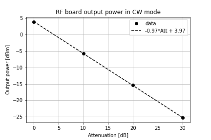
We can’t accurately predict from this plot how much power will leave the antenna port of our radio – the amplifier gain will vary a bit from build to build and band to band, as will the passband loss of the BPF and LPF filters.
So the calibration process is fairly simple: for a desired output power, measure what attenuation value results in this power at the output of the radio in each band. You can then change the power to a specified value based off this known data point by changing the attenuation by a known amount.
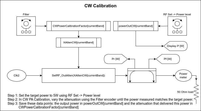
The process is shown in the diagram above: set the calibrated power level using the RF Set -> Power level menu, and save this in the variable powerOutCW[currentBand]. This value should be 5 W to stay in the linear regime of the amplifier.
Then, in the CW PA Calibration menu, vary the attenuation until the power leaving the radio, as measured using an external power meter, matches this setting. The attenuation level that resulted in this power is saved in CWPowerCalibrationFactor[currentBand].
Then, if we change the value of the attenuator we can calculate the new transmitted power as:
\[P = P_{\rm cal} 10^\frac{A_{\rm cal} - A}{10}\]where \(P_{\rm cal},A_{\rm cal}\) are the power and attenuation we identified above and \(A\) is the attenuator setting in dB. Or, in code, as:
transmitPowerLevelCW = powerOutCW[currentBand] *
    pow(10, (CWPowerCalibrationFactor[currentBand] - attenuation )/10.0 );
Alternatively, if we want to change the power level we can calculate the attenuation that will deliver this power according to:
attenuation = CWPowerCalibrationFactor[currentBand]
    - 10*log10f(transmitPowerLevelCW / powerOutCW[currentBand]);
This is shown in a diagram below: changing the output attenuation updates the calculation of the power being transmitted, and changing the value of the power being transmitted updates the attenuator setting.
![]()
SSB Power Level Calibration
SSB calibration is very similar, except that we use a tone generated in the DSP code of the transceiver when performing the calibration:
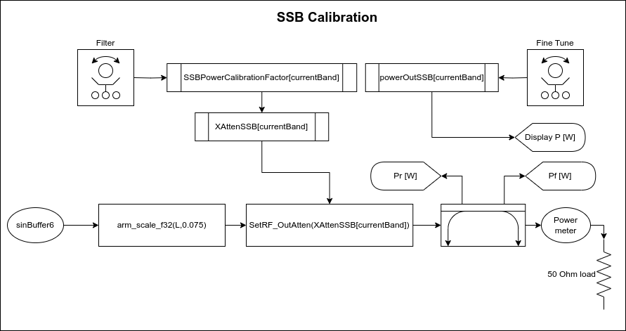
There is one more factor to pay attention to in SSB calibration, which is the microphone gain. The calibration process uses a fixed amplitude sinusoidal tone. But every radio may have a different microphone, and every user will have a different voice. So after the power level is set using the sinusoidal tone you then need to set the microphone gain such that your normal speaking voice delivers the power level you want.
Power and SWR Measurement Calibration
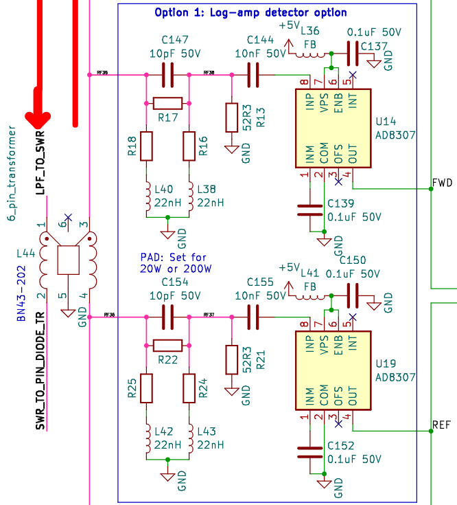
The LPF control board for the T41 contains a circuit that measures the forward power and the reverse power. This allows us to measure the power we’re transmitting, and to calculate the SWR on the transmission line. The relevant bit of circuitry is excerpted below:
Power measurement errors
After some attenuation through the directional coupler and attenuator pads, the signal is measured by AD8307 logarithmic amps. These devices produce an output voltage proportional to their input power according to the following formula (in the ideal case):
\[V_{\rm out} [{\rm mV}] = 25(P_{\rm in}[{\rm dBm}] + 84)\]In the recommended configuration for a 20W radio, the coupler and attenuator between them will reduce the signal amplitude by 46 dB, so \(P_{\rm in}[{\rm dBm}] = P_{\rm TX}[{\rm dBm}]-46\). We can therefore calculate the power on the transmission line from the voltage out of the AD8307 according to this formula:
\[P_{\rm TX}[{\rm dBm}] = \frac{V_{\rm out} [{\rm mV}]}{25} - 84 + C [{\rm dB}]\]where \(C\) is the coupler + attenuator value of 46 dB (or whatever).
However, that’s not quite right. The AD8307 devices has two errors that need to be compensated for in the calibration process. The first is an error in the slope, which is nominally 25 mV/dB, but can vary from 23 to 27. The second is an error in the offset, which is nominally -84 dBm but can vary from -87 to -77, according to the datasheet. The formula relating the transmission line power to output voltage is actually:
\[P_{\rm TX}[{\rm dBm}] = \frac{V_{\rm out} [{\rm mV}]}{25+e_s} - 84 +e_i + C [{\rm dB}]\]Here, \(e_s\) is the error term in the slope and \(e_i\) is the error term in the intercept.
Power measurement calibration
Let’s see this in practice. The plot below shows how the output voltage of the forward path AD8307 varies as I increase the attenuation from its nominal setting. The radio was in CW mode. As expected, the output voltage drops as the attenuation is increased.
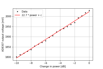
Also plotted is the best-fit slope. The slope of this line should be 25 mV/dB – in reality I measure 22.7 mV / dB. So the slope error term is \(e_s = -2.3\). We repeat this process in each of the bands to measure the slope intercept:
- Configure for CW mode with the nominal band attenuation setting. Measure the voltage out of the AD8307.
- Increase the attenuation in 0.5 dB steps, measuring the AD8307 output at each step.
- Perform a least-squares fit to the line formed by (attenuation, voltage) points, obtaining the slope \(m\).
- Calculate the error term \(e_s = m-25\).
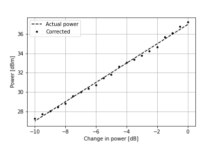
Once we have performed the CW Power Amp calibration we can also calculate the intercept error term \(e_i\). Let’s calculate what we think the power is, including the slope intercept we just calculated:
\[\begin{aligned} P_{\rm out} & = \frac{V_{\rm out} }{25-2.3} - 84 + 46 + e_i \\ & = \frac{2028}{22.7} -38 + e_i \\ & = 51.34 + e_i \\ \end{aligned}\]At the band’s calibrated power setting, we know that the output power is actually 5W, which is 36.99 dBm. So we can then calculate the intercept offset:
\[\begin{aligned} 36.99 & = 51.34 + e_i \\ \therefore e_i & = 36.99-51.34 \\ & = -14.35 \\ \end{aligned}\]We can repeat this calculation using all the other attenuation values and calculate the average intercept offset. The comparison of the corrected power and the predicted actual power is shown in the plot below:
SWR calibration
So now we have a method to correct the power measurement. This is easily done for the forward power measurement circuit as we can use an external power meter with a 50 Ohm dummy load on its output. For the reflected power measurement circuit, we need to have a signal of known power reflected back into the radio. We achieve this by using a dummy load that is not at 50 Ohms.
How much power is reflected if I use, say, a 100 Ohm dummy load? The reflection coefficient is then:
\[\begin{aligned} \Gamma &= \frac{Z_L-Z_0}{Z_L+Z_0} \\ &= \frac{100-50}{100+50} \\ &= \frac{1}{3} \end{aligned}\]The SWR is:
\[\begin{aligned} SWR &= \frac{1+|\Gamma| }{1-|\Gamma|} \\ &= 2 \end{aligned}\]And finally the reflected power is:
\[\begin{aligned} P_R &= P_F \Bigg( \frac{SWR-1}{SWR+1} \Bigg)^2 \\ &= P_F \Bigg( \frac{1}{3} \Bigg)^2 \\ &= \frac{P_F}{9} \end{aligned}\]Therefore, if we connect a 100 Ohm dummy load to the antenna output, we can use the power measurement calibration approach described above to calibrate the reflected power measurement circuit too.
Making a good dummy load
A brief aside on making a good dummy load. For the purposes of this test the dummy load should be purely resistive. You might be tempted to use a resistor like those in the photo below – these are capable of supporting a high power load and can be picked up cheaply at hamfests.
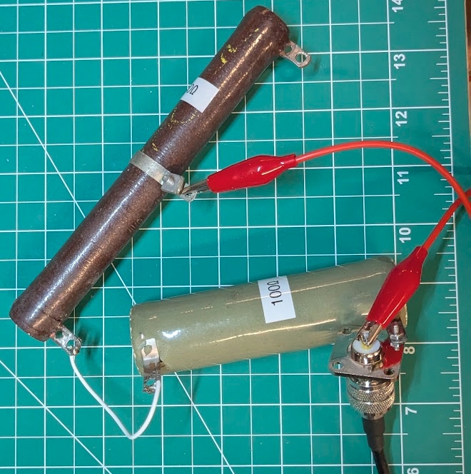
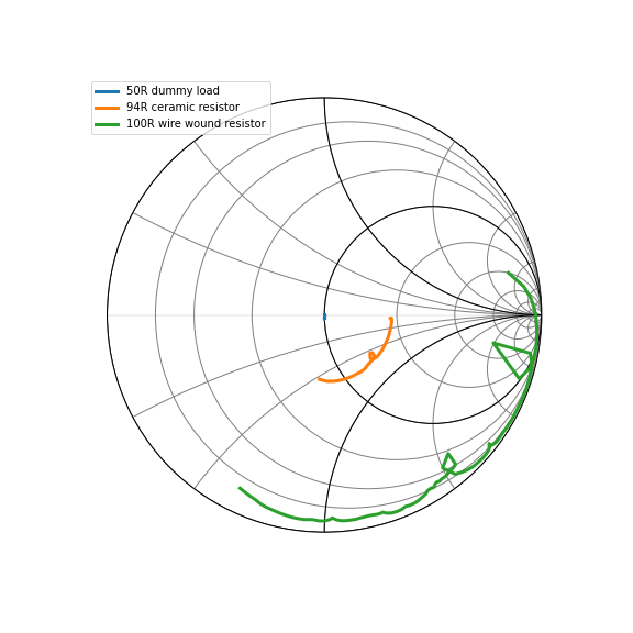
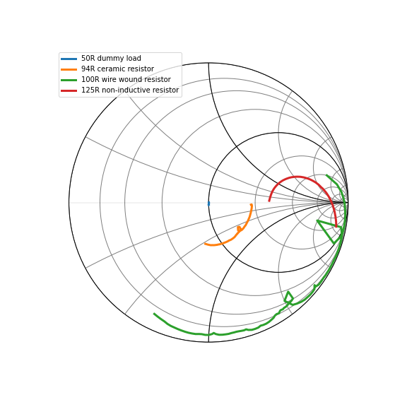
However, these are wirewound resistors, which means that, while they might be a resistor at DC, at HF frequencies they have a substantial inductance. This can be see on a Smith chart – the chart below compares a ~100 Ohm ceramic resistor to a wirewound resistor of the same DC resistance. The VNA swept from 1 to 60 MHz, and you can see that the impedance of the wirewound resistor is substantially higher than 100 Ohms over this whole range.
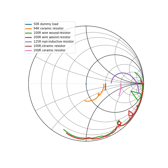
To make a dummy load capable of sinking many watts of power, you might think that you need to use non-inductive wirewound resistors. However, these might not deliver the expected performance. I bought some precision non-inductive wirewound resistors on Amazon and found that they did not behave like pure resistors. The Smith plot below shows that the 125 Ohm non-inductive resistor does not behave like a 125 Ohm resistor between 1 and 60 MHz.
To create an actual resistive load I used these thick film ceramic resistors. These had the expected behavior over the 1 to 60 MHz range.
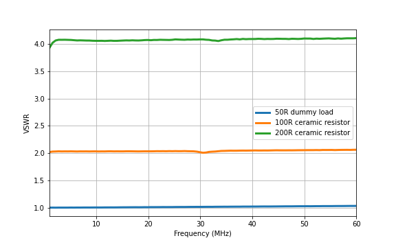
Plotting the VSWR, I get the expected performance (note that VNA was not accurately calibrated for this measurement).
| \(Z_L [\rm Ohms]\) | \(\Gamma\) | SWR | \(P_R / P_F\) |
|---|---|---|---|
| 50 | 0 | 1 | 0 |
| 100 | 1/3 | 2 | 1/9 = 0.333 |
| 200 | 3/5 | 4 | 9/25 = 0.36 |