Introduction
A VSWR meter is an important part of any amateur radio station. It measures how well matched your antenna is and measures your transmitted power.
The goals for the device I want to build are:
- Measure VSWR.
- Measure output power up to 100 W power level limit.
- 3 MHz to 30 MHz operation.
- Use the Raspberry Pico and OLED display I had laying around.
Credit: thanks to G3TXQ for sharing his SWR meter design and schematic diagram. Thanks to N7DDC for sharing the design of the ATU-100 antenna tuner. And to W2AEW for his excellent explanation of how a directional coupler works. K6JCA’s website is a treasure trove of information. IN3OTD has an online calculator for synthesizing arbitrary resistor values from standard value. All these were tremendously helpful as I designed my own VSWR meter.
TL;DR The finished design
The KiCad design files, gerber files, and PDF export of the schematic diagram of my VSWR/Power meter can be found on Github and below.
Principle of operation
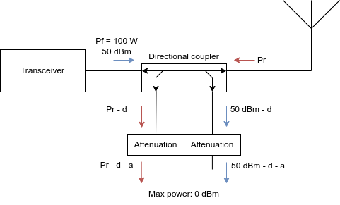
The meter works by measuring the power in the forward-traveling wave (the signal produced by the transceiver) and in the reverse-traveling wave (the signal reflected by the antenna). These measured powers can then be used to calculate the standing wave ratio. A block diagram view of the system looks like this:
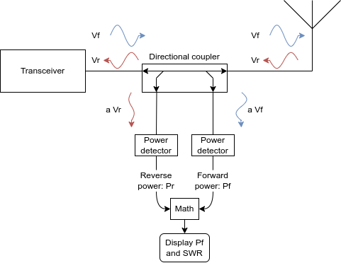
The component that neatly separates the forward and reverse traveling waves on the transmission line between the transceiver and antenna is a directional coupler. W2AEW has an excellent explanation of how a directional coupler works on Youtube. Directional couplers separate some small fraction of the forward and reverse waves, indicated by the attenuation constant a in the diagram.
Once we’ve measured the power in the forward and reverse waves, we calculate the SWR according to this formula:
\[\mathbf{SWR} = \frac{1 + \sqrt{P_r/P_f}}{1 - \sqrt{P_r/P_f}}\]We can then display the calculated value on a screen.
System sections
I’ll walk through the system design starting at the “end” - the microprocessor and screen - and work back towards the beginning.
Microprocessor and screen
I had a stack of Raspberry Pico development boards and some SSD1306 128x64 pixel OLED displays in my parts drawer, so I decided to use them to calculate the SWR and display it on screen. The complex parts of this section are all in code, which is discussed below in the Pico micropython code section. The only impacts of this design decision on the rest of the system are:
1) The output of the power detector stage is limited to 3.3 V.
2) We will need a 3.3 V supply rail.
Power detector
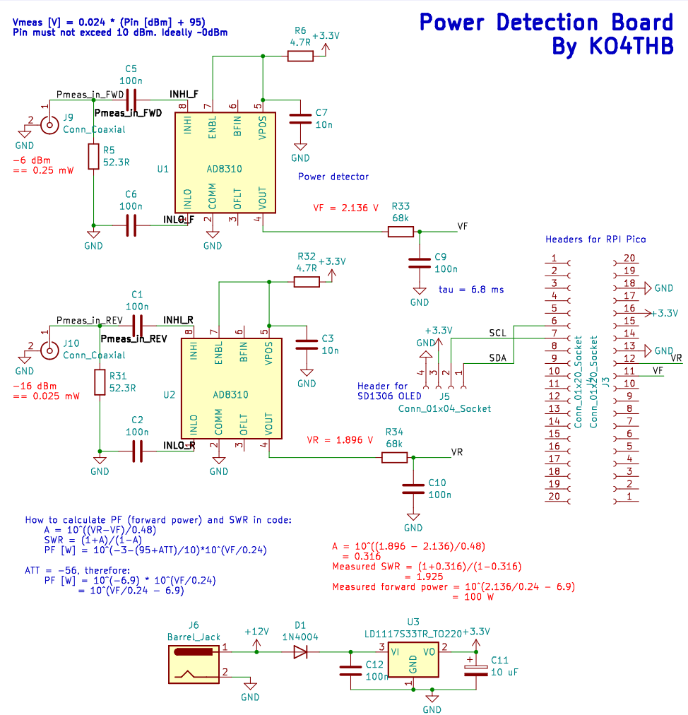
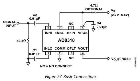
I decided to base the power detector on the AD8310 logarithmic amplifier. The term “logarithmic amplifier” is… confusing to the uninitiated. For our purposes, it produces an output voltage proportional to the input power. The datasheet provides a schematic diagram that’ll work for our purposes.
The AD8310 is designed to work between -90 dBV and 0 dBV. Its output will range from ~0.4 V at the lower limit up to ~2.6 V at the upper limit according to this response curve.
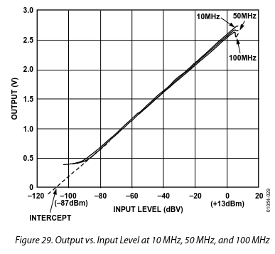
Values in dBV are converted to dBm by adding 13 dB; see the datasheet’s Table 4 for a more nuanced discussion on this topic. For our purposes, we can simply state that our design must ensure that the maximum input power to the power detector does not exceed +10 dBm (10 mW). If we stick to this, the relationship between the output voltage (in units of Volts) and input power (in units of dBm) is:
\[V_{\mathrm{out}} [\mathrm{V}] = 0.024 ( P_{\mathrm{in}} [\mathrm{dBm}] + 95)\]Combining the power detector and display stages, we end up with this schematic:
I’ve added a circuit based on the LD1117S33 linear voltage regulator to supply 3.3V to the Pico and the AD8310. I also added a smoothing low-pass filter to the outputs of the AD8310’s - these smooth out rapid changes in measured power and allow the microcontroller to more accurately measure them at a slower sample rate.
To stay safely below the 10 dBm input limit of the AD8310 power detector, we’ll impose a requirement on the directional coupler section that:
3) The output of the directional coupler section must not exceed 0 dBm (1 mW).
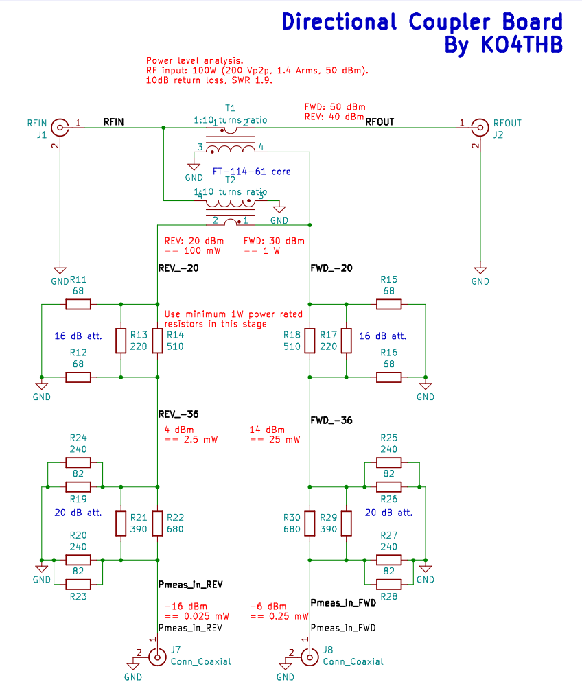
Directional coupler
This section of the circuit extracts “some fraction” of the power flowing in both directions on the transmission line. At this point we hark back to our design condition of 100 W maximum transmit power. If we have 100 W (50 dBm) of power flowing in the forward direction, we want the amount of power delivered to the power detector to be no more than 1 mW (0 dBm). So the coupling factor for this section must be at least -50 dB.
Transformer turns
Directional couplers are built using transformers where the primary winding has one turn and the secondary winding has N turns. The coupling factor is then given by:
\[\mathrm{Coupling\ factor\ [dB]} = -20 \log_{10}(N)\] \[N = 10^{\frac{\mathrm{Coupling\ factor\ [dB]}}{-20}}\]So if we want to get our coupling factor of -50 dB out of the transformer alone, we will need 316 turns on the secondary. This is too many turns.
A better approach is to build a directional couple with a “reasonable” number of turns on the secondary coil, and use attenuators to reduce the power level. “Reasonable” is up to you and your aching fingers to decide, but I’d prefer to keep it less than 20.
I decided to use 10 turns, which gives me a coupling factor of d = -20 dB. I then need at least 30 dB of attenuation to reduce the power to the required level.
Attenuators
Attenuators are easy to build using Pi resistor circuits. There are many online calculators that will give you the appropriate resistor values to achieve a specified attenuation level. A design consideration to pay attention to is the amount of heat the resistors will need to safely dissipate. In our case, the attenuators will take 30 dBm (1 W) of input power and reduce it to 0 dBm (1 mW), dissipating the difference of 0.999 W as heat.
I opted to split the attenuator into two stages of attenuation: 16 dB followed by 20 dB. I also used parallel resistors to more accurately achieve the required resistor values. IN3OTD has a great online calculator that will help you find the right combinations of standard resistor values. I opted to use the E24 series, which worked well enough.
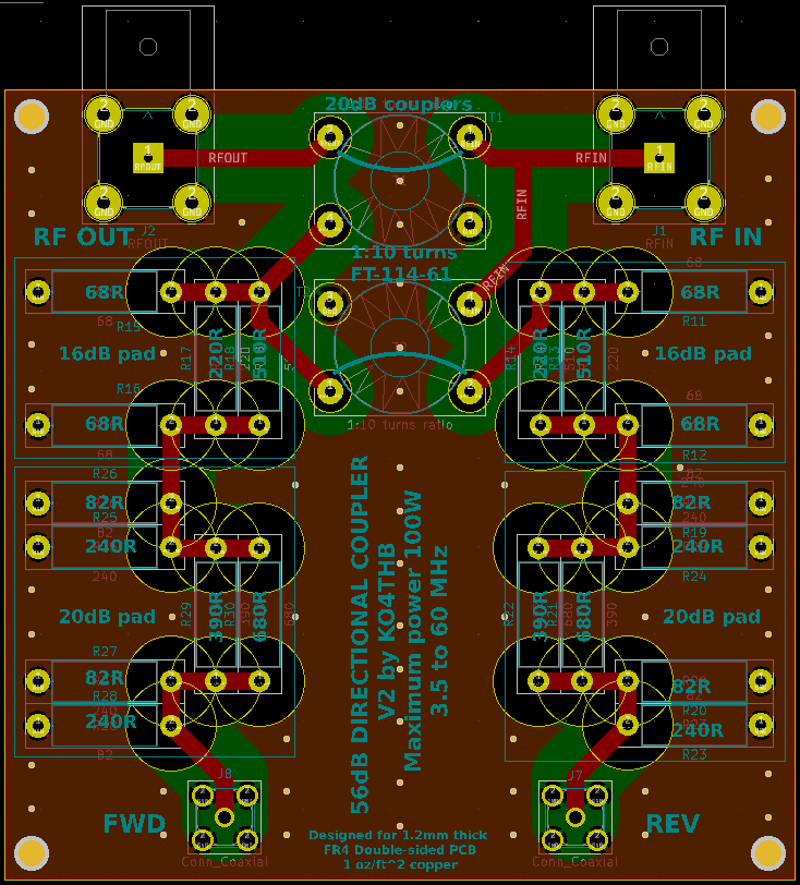
The final schematic for this section of the circuit is:
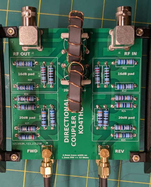
Board layout
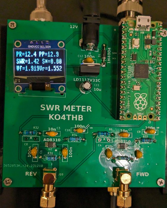
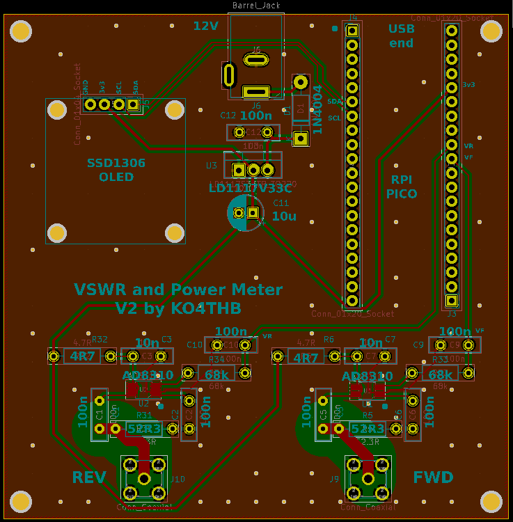
I used KiCad to lay out the circuit on two 1.2 mm thick two-layer boards. The components were arranged so that the boards could be stacked for more compact packaging.
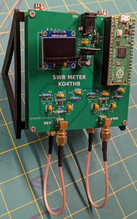
The final assembled system looks like this:
Pico micropython code
The microcontroller samples the voltages produced by the power detector stages and does the math for converting them to equivalent powers, and calculating the SWR. I measure the voltage in two ways: the peak voltage observed during the measurement window and the RMS voltage. The peak voltage is relevant for regulatory reasons: the Peak Emitted Power (PEP) of the station is limited by law. The RMS voltage measurement might be useful to know too - I measure it because I can, not because I have a particular reason for doing so.
The Pico is configured to run micropython. This is the code running on it. The external ssd1306 library I used was this one. The other libraries are part of standard micropython.
import machine
import utime
from machine import ADC
from ssd1306 import SSD1306_I2C

# Display configuration
sda=machine.Pin(4)
scl=machine.Pin(5)
i2c=machine.I2C(0,sda=sda, scl=scl, freq=400000)
oled = SSD1306_I2C(128, 32, i2c)

# ADC configuration
# GPIO 26 == ADCf == board pin 31
# GPIO 27 == ADCr == board pin 32
ADCf = ADC(26)
ADCr = ADC(27)
# Attenuation between TX line and detector in dB
ATT_dB = -56
# only calculate SWR if forward power is greater than this
power_threshold_W = 0.5

oled.text("KO4THB", 30, 0)
oled.text("SWR Meter", 10, 10)
oled.text("100 W max",10,20)
oled.show()

utime.sleep(5)

def read_and_average(ADCf,ADCr,N=100):
    # Read the ADC inputs the specified number of times.
    # Return the RMS and Peak (FWD only) voltages measured.
    # 100 iterations of this function takes 3.5 ms
    smf = 0
    smr = 0
    pkf = 0
    for k in range(N):
        f = ADCf.read_u16()
        smr += (ADCr.read_u16())**2
        smf += f**2
        if f > pkf:
            pkf = f
    return (smf/N)**(0.5) * 3.3 / 65536, (smr/N)**(0.5) * 3.3 / 65536, pkf* 3.3 / 65536

def measure_swr():
    # This will take almost half a second
    Vf_RMS,Vr_RMS,Vf_peak = read_and_average(ADCf,ADCr,10000)

    Pf_RMS_W = 10**( Vf_RMS/0.24 -3 -(95+ATT_dB)/10)
    Pf_peak_W = 10**( Vf_peak/0.24 -3 -(95+ATT_dB)/10)

    A = 10**((Vr_RMS - Vf_RMS)/0.48)
    # Also calculate an "inaccurate" SWR for low power testing purposes
    if Pf_peak_W > power_threshold_W:
        SWR = (1+A)/(1-A)
        SWR_inac = 0.0
    else:
        SWR = 0.0
        SWR_inac = (1+A)/(1-A)

    return Pf_RMS_W, Pf_peak_W , SWR, SWR_inac, Vf_RMS, Vr_RMS

while True:
    Pf_RMS,Pf_peak,swr,swr_inac, Vf, Vr = measure_swr()
    # Flash the LED
    machine.Pin(25, machine.Pin.OUT).value(1)
    utime.sleep(0.05)
    machine.Pin(25, machine.Pin.OUT).value(0)

    oled.fill(0)
    oled.text("PR=%2.1f"%Pf_RMS, 0, 0)
    oled.text("PP=%2.1f"%Pf_peak, 64, 0)
    oled.text("SWR=%3.2f"%swr, 0, 10)
    oled.text(" S*=%3.2f"%swr_inac, 64, 10)
    oled.text("Vf=%4.3f"%Vf, 0, 20)
    oled.text("Vr=%4.3f"%Vr, 64, 20)
    oled.show()
Testing
Coupling factor
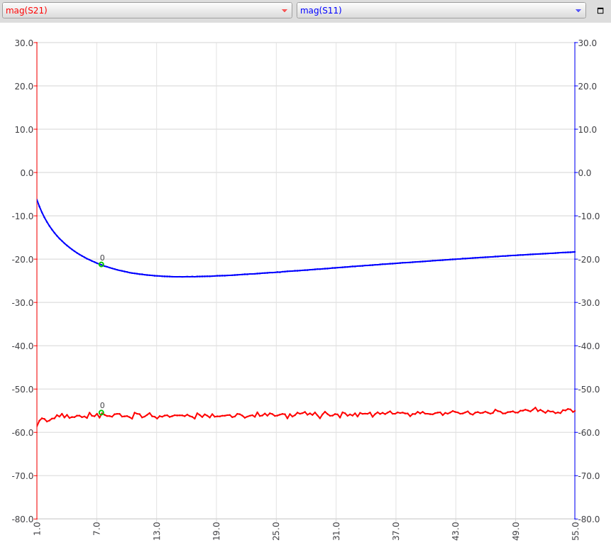
The coupling factor of the directional coupler board should be -56 dB. The factor, as measured with a NanoVNA, meets this value over the desired band. The blue trace is Return Loss, and the red trace is Coupling Factor. Frequency span is 1 MHz to 55 MHz.
SWR accuracy
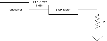
I tested the measured SWR by terminating the output of the SWR meter with a variety of resistor values. By varying the value R of the resistor, I can change the SWR of the circuit in a predictable way. The SWR varies with resistance R as follows:
\[\Gamma = \frac{ R - 50 }{R + 50 }\] \[\text{SWR} = \frac{ 1 + |\Gamma| }{ 1 - |\Gamma| }\]I only had low power (1/4 W) resistors on hand for the test, so my transceiver output was very low, only 7 mW, for the test.
This method of measuring SWR accuracy has a significant shortcoming; it assumes that my transceiver’s output impedance is exactly 50 Ohms (this is baked into the SWR equation above). I’m sure that my transceiver’s output impedance isn’t exactly this, but it’s the best I can do for now. I’ll see if I can come up with a better measurement method in the future.
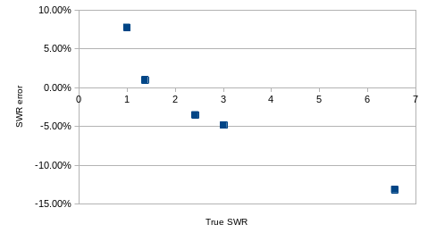
Regardless, the results are tabulated and plotted below. Better than 5% accuracy for “low” VSWRs of less than 3.0. I’m pretty happy with this!
| R [Ohms] | True SWR | Vf [V] | Vr [V] | SWR measured | SWR error |
|---|---|---|---|---|---|
| 50 | 1 | 1.125 | 0.44 | 1.08 | 7.77% |
| 68.7 | 1.374 | 1.119 | 0.74 | 1.39 | 0.99% |
| 120.9 | 2.418 | 1.097 | 0.906 | 2.33 | -3.50% |
| 150.4 | 3.008 | 1.088 | 0.936 | 2.86 | -4.81% |
| 327.7 | 6.554 | 1.072 | 0.998 | 5.69 | -13.14% |