Introduction

The transmit power calibration process for the T41 software defined transceiver involves figuring out how to control the signal levels at various points in the receiver to result in transmitting a known amount of clean power. The clean part is critical: if you try to send too much power through active elements like mixers and amplifiers you get intermodulation distortion which muddles the sound quality and transmits signals out-of-band.

This blog post describes how I went about characterizing the T41 V12 hardware. First, here is a simplified schematic of the transmit chain of the T41 radio:

For single sideband mode, a microphone is attached to the main board where its signal is digitized and processed in the DSP code. The output from the main board takes the form of baseband I/Q signals on the IQ Output connector. These signals flow to the RF board where they are moved to the transmit frequency by a mixer. We then control their power level using a variable attenuator. The RF board output is amplified by the K9HZ amplifier (I’ve omitted the bandpass filter from the diagram) and filtered by a low pass filter (LPF). The output of the LPF goes to the antenna connector.

When we’re transmitting CW, an RF tone is instead injected directly into the attenuator – the DSP chain and mixer are not used. The RF tone is generated by the Si5351 chip on the RF board.

All this testing was done using Version 66-9 of the code, this commit in particular.

Gain

First, we’ll characterize the gain of the transmit path: how the amplitude of a sinusoidal tone changes as it moves through the various stages of the transmit path.

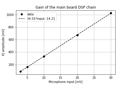
Main Board: Microphone Input to IQ Output

I connected an audio signal generator to the mic inputs on the Teensy audio hat. The audio generator produced a 1 kHz tone at a range of voltage amplitudes. I used a Digilent Analog Discovery 2 (AD2) to produce the signal. It was controlled by the Digilent Waveforms software.

I connected the oscilloscope inputs of the AD2 to the IQ output of the main board to measure the amplitude of the IQ signals produced in response to this microphone input. The plot below shows how the IQ voltage amplitude out of the main board depends on the microphone input.

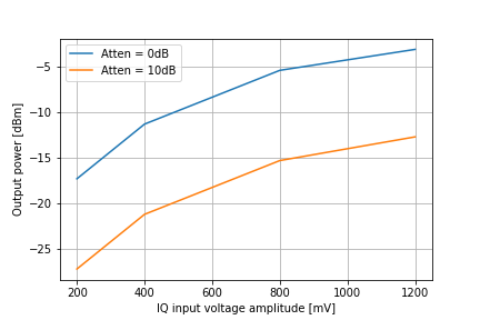
Microphone input to IQ output and best-fit line

RF Board: SSB IQ input to RF output

In this test I connected the AD2 to the IQ input of the RF board. The AD2 was configured to generate two sinusoids 90 degrees out of phase to form a quadrature pair. A spectrum analyzer was connected to the RF output of the board to measure the power of the resulting tone. The results are shown below for two different settings of the attenuator.

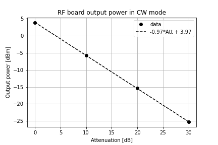
Input voltage to output power for RF board

RF Board: CW Power Levels

How does the power out of the RF board change as the attenuator value is varied? I connected the RF board output to a spectrum analyzer, tuned the T41 to 14.1 MHz, and measured the output power at a range of attenuator settings. The data points and the best-fit line are shown below. With no attenuation the RF board produces +3.9 dBm and the level reduces proportionately as the attenuation is increased.

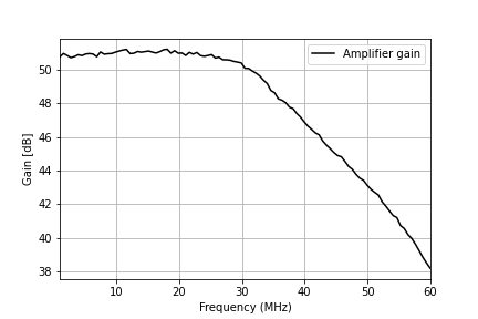
Power of a 14.1 MHz tone and best-fit line

Amplifier

I measured the gain of the amplifier using a NanoVNA with 40dB of attenuation on the transmit port. The gain vs frequency is shown in the plot below. This is measured between the input and output SMA terminals of the K9HZ amplifier.

K9HZ gain vs frequency

To measure the power output of the radio given different RF board power output levels, I used the CW tone generator on the RF board to generate outputs of known power, based on the previously-characterized relationship between RF board attenuation and RF board CW output power.

The RF board was connected to the amplifier through the LPF control board, so this measurement includes the BPF passband attenuation and any cable / switch / connector losses. I measured the output power at the antenna port using a spectrum analyzer with a 20dB directional coupler and 40dB of attenuation in front of it (60dB total). The measurement was performed at 14.1 MHz.

Amplifier power in vs power out

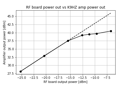
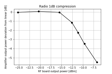
This shows that the amplifier starts to compress when the output power exceeds roughly 5 W. If we remove the best-fit straight line from the linear part of the curve we find that the point at which the radio’s output power drops by 1dB from the expected power – the 1dB compression point – occurs when the RF board’s output reaches roughly -13dBm.

K9HZ 1dB compression point

Pulling it all together

To avoid gain compression, I conclude that we need to keep the RF board’s output power below -15 dBm. This translates to:

In CW mode, keep the attenuation of the RF board greater than 20 dB.
In SSB mode, keep the IQ outputs of the main board below approximately 250 mV when the attenuation is 0dB.
This means keep the microphone amplitude below approximately 7.5 mV with the default mic gain settings and my particular microphone.

However, as we’ll see below, we need to impose different limits if we also want to keep the intermodulation distortion of the signal at acceptable levels.

Intermodulation Distortion (IMD)

Measurement method

IMD is measured by injecting two tones into the test setup simultaneously. A perfect system would reproduce those two tones at the output, each output tone a scaled or shifted version of its input as if the other tone were not there. An imperfect system produces the two desired tones as well as undesirable new tones generated by combining the input tones in various ways. When we measure IMD we want to know how strong these intermodulation products are compared to the two desired tones. We usually use tones at 700 and 1900 Hz when testing amateur radio equipment.

The waveforms software that controls the AD2 is capable of playing arbitrary waveforms on its output. You provide it these waveforms in a CSV file. I used the following Python code to generate a 20ms long snippet of I/Q data containing two tones.

import numpy as np

duration_s = 0.02
sample_rate_Hz = 192000
tone1_Hz = 700
tone2_Hz = 1900

Nsamples = duration_s * sample_rate_Hz
t = np.arange(0,Nsamples)/sample_rate_Hz
i1 = 0.5*np.sin(2*np.pi*tone1_Hz*t)
i2 = 0.5*np.sin(2*np.pi*tone2_Hz*t)
is = i1+i2

q1 = 0.5*np.cos(2*np.pi*tone1_Hz*t)
q2 = 0.5*np.cos(2*np.pi*tone2_Hz*t)
qs = q1+q2

np.savetxt("two_tone_700-1900_Hz_192000ksps_0.02s-I.txt",is)
np.savetxt("two_tone_700-1900_Hz_192000ksps_0.02s-Q.txt",qs)

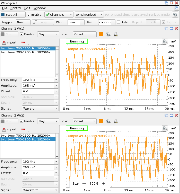
I then configured the wavegen function in the waveforms software to read these files and play them on the W1 and W2 channels as shown below. Note that I reduced the amplitude of the W1 channel compared to the W2 channel – this is to compensate for gain imbalances between the I and Q channels on my RF board that lead to poor image rejection. In all the tests I performed below the stated amplitude is that of the W2 channel and the W1 channel is always 84% of the W2 channel.

Screenshot of the wavegen function in Digilent Waveforms generating a two tone signal

I injected these signals into the IQ input of the RF board and measured the following intermodulation products:

Third order IMD is at 2*f1-f2 and 2*f2-f1 = -500 Hz and 3100 Hz
Another tone appeared at -3300 Hz, which doesn’t correspond to a particular known intermodulation product.

RF Board

The IMD for the RF board is shown in the plot below. Note how the level of attenuation does not affect the IMD – this implies that the IMD results from the IQ phasing amplifiers or the mixer on the RF board.

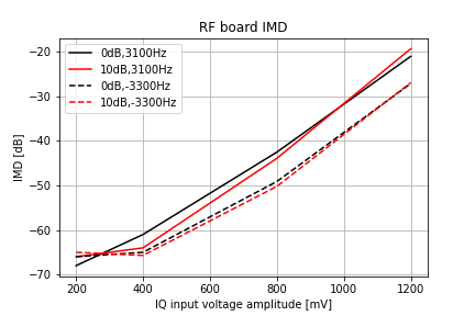
Comparing this plot to the recommendations in the gain section, we see that if we follow the guidance to keep the IQ inputs to the RF board below 250 mV, the RF board will not generate IMD products stronger than -65 dB, which is excellent.

RF Board plus Amplifier

However, what matters is not the RF board but the whole radio, which includes the amplifier.

Using the same measurement technique outlined above, but injecting the IQ signal into the IQ input of the RF board and measuring the output on the radio’s antenna connector, we find the relationship between the third order IMD ratio and the output power.

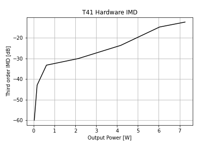
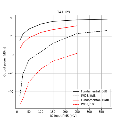
This is usually plotted to show how the power in the fundamental and the power in the IMD products grow as the input power in varied. Data are plotted for two different attenuator settings.

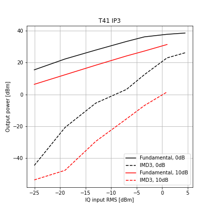
A note on the input power: it was calculated from the IQ voltage amplitude according to the following formula:

\[P [W] = \Bigg( \frac{V_{\rm amp} [V]}{2} \Bigg)^2 \frac{1}{50}\]

The RMS voltage of a single tone is \(V_{\rm amp} / \sqrt{2}\). We have two tones of equal amplitude, so the RMS voltage due to both tones being present simultaneously is \(V_{\rm amp} / 2\).

If we plot the same data with units of RMS voltages on the x axis, we get the following: