Introduction

A quadrature sampling detector is a common way of selecting and digitizing a portion of the electromagnetic spectrum. This post walks through the math to explain how it works, and then analyzes in detail an implementation commonly found in amateur radio equipment. We start by discussing the design of a simple mixer, which motivates the need for quadrature mixing in a quadrature sampling detector.

Background: a basic mixer

In this section I walk through describing a simple mixer. It’s helpful to start with a simpler example when introducing the terminology and conventions I’ll be using.

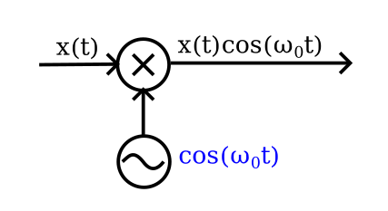
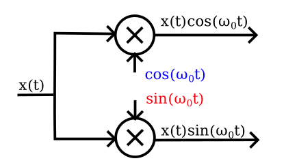
Consider a multiplier, shown above. An input voltage \(x(t)\) is multiplied (never mind how for now) with a sinusoidal voltage called a local oscillator at some frequency \(\omega_0\). The output voltage from the multiplier is then \(x(t)\cos(\omega_0 t)\).

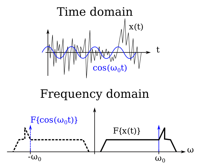
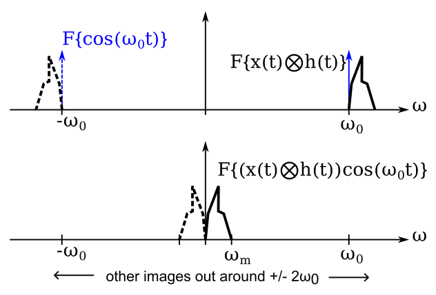
The plots above show what these signals look like in the time and frequency domains. In the time domain, I’ve shown \(x(t)\) as some arbitrary noisy signal. \(\cos(\omega_0 t)\) is a sinusoid. It’s very useful to look at the frequency domain representation of the signals as well. In this case, the cosine wave is simple: single tones at the frequencies \(+\omega_0\) and \(-\omega_0\). The notation \(F\{a\}\) means the Fourier transform of \(a\). As shown by the shape of \(F\{ x(t) \}\), \(x(t)\) consists of contributions from a wide range of frequencies, with a peak just above \(\omega_0\) which is our signal of interest in this example – the band we’re interested in. I’ve shown the positive frequency components of each signal with solid lines and the negative frequency components with dashed lines – this is useful later.

What does the output of the mixer look like in the frequency domain? That’s shown by the plot below. Remember that multiplication in the time domain is equivalent to convolution in the frequency domain, and convolving a signal with an impulse has the effect of shifting it in frequency.

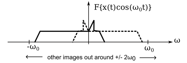
Can you spot the problem? The signal we’re looking for (the little bump in the spectrum) now overlaps with part of the negative frequency image. This is no good. At best it adds unwanted noise to our measurement. At worst there may be strong signals at the negative frequency which will overwhelm our band.

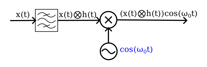
The solution is to filter \(x(t)\) before we multiply it with the local oscillator, as shown below. Here \(h(t)\) represents the action of the filter on \(x(t)\), and the signal that is mixed is the convolution of the two: \(x(t) \bigotimes h(t)\).

The output of the mixer is now shown below. Much nicer! No overlap between positive and negative frequency images, and ready for onward manipulation and digitization.

To digitize this signal we need a single ADC running at a sample rate of at least \(2\omega_m\), where \(\omega_m\) is the maximum frequency present in the signal.

That’s all well and good, but there are two principle shortcomings of this mixer:

1. You need a (comparatively) fast ADC and digital logic.
2. It only works at one LO frequency! If you change the frequency of the LO \(\omega_0\), you also need to change the filter. Since tunable filters are hard / expensive / don’t work as well, this effectively means that you need a separate LO + mixer + filter for every band you want to sample.

Solution: the quadrature mixer

A quadrature mixer (the RF part of the quadrature sampling detector) solves the problems of the simple mixer at the expense of a more complicated mixing stage. The block diagram view of a quadrature sampling detector is shown in this figure. I’ve added the digitization step and some of the digital signal processing steps.

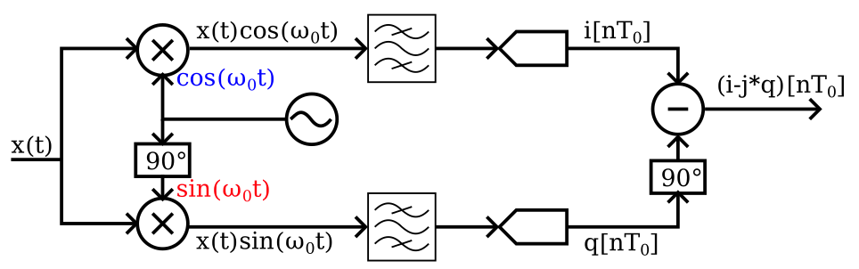
The input signal \(x(t)\) is split and multiplied (i.e., mixed) with a local oscillator (LO) at frequency \(\omega_0\), with one part of the split being multiplied directly and the other with a \(90^\circ\) phase shift first applied to the LO signal. These two signals, \(i(t) = x(t) \cos(\omega_0 t)\) and \(q(t) = x(t) \sin(\omega_0 t)\), are then filtered by anti-aliasing filters before being digitized to form digital signal streams \(i[nT_0]\) and \(q[nT_0]\) respectively (\(T_0 = \frac{2\pi}{\omega_0}\)). These quadrature streams are combined with another phase shift and a difference to form the output stream \(i[nT_0] - j q[nT_0]\), where \(j = \sqrt{ -1}\). This output stream is made up only of the positive frequency spectral component of \(x(t)\), which solves the overlap problem we encountered above. How? (But first note how the quadrature mixer only has a fixed anti-aliasing filter after the mixer, not before. We can change the LO frequency without needing new filters. Problem solved!)

First, let’s take a look at the spectral representation of the input signals to the multipliers. \(F\{ a \}\) indicates the Fourier transform of \(a\). I’ve added the imaginary axis – signals are represented by complex numbers in the frequency domain.

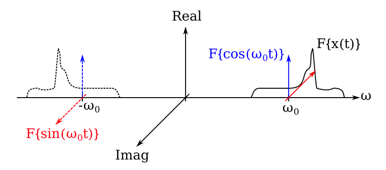
The input signal \(x(t)\) covers some band that spans either side of the LO frequency \(\omega_0\). The positive frequency component (or image) of each signal is represented by a solid line and the negative frequency by a dashed line. For simplicity, we’ve assumed that the imaginary component of \(F\{ x(t) \}\) is zero.

After the output of the multipliers, the signals \(i(t)\) and \(q(t)\) have the following spectra – remember that multiplying in the time domain is equivalent to convolving in the frequency domain. These figures omit the higher frequency images around \(\pm 2\omega_0\) for simplicity.

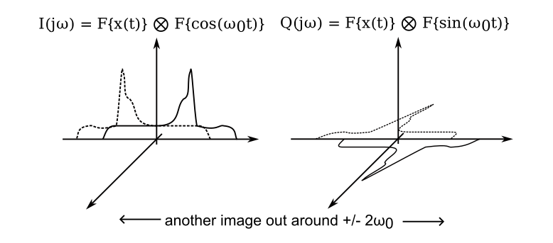
These signals are filtered by anti-aliasing filtered and digitized to form digital signal streams. Multiplying the digital stream \(q[nT_0]\) by \(j\) has the effect of rotating it by \(90^\circ\) in the complex plane. The positive and negative frequency components now have opposite signs, and therefore adding or subtracting \(i[nT_0]\) and \(jq[nT_0]\) has the effect of returning the negative or positive frequency components of \(x(t)\) respectively, as shown in the figure below.

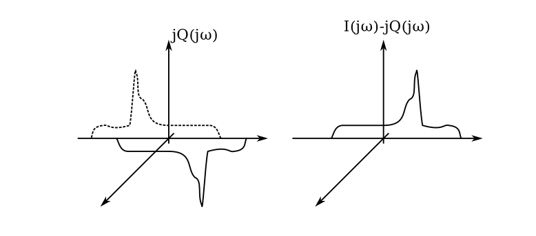
Put another way, both \(i[nT_0]\) and \(jq[nT_0]\) individually suffer from the same overlapping-negative-frequency problem that the simple mixer had, but with a phase difference between the positive and negative frequency components. This allows us to remove the negative frequency image by subtracting one from the other. Neat!

How do I actually build one?

To make a quadrature mixer we need electrical circuits to do two things:

1. To generate an LO signal and phase shift it by \(90^\circ\).
2. To multiply our signal \(x(t)\) with the LO signals.

A very popular way of generating the LO signal at HF frequencies is to use the Si5351A (and equivalent) programmable clock generator. This device is can generate any frequency up to 160 MHz on any of its outputs with 0 ppm error. It can be programmed via an I2C interface to simultaneously generate square wave signals separated by \(90^\circ\) in phase, as shown below.

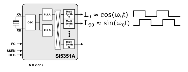
A square wave is not sinusoidal, that’s true, but the rest of the system design can eliminate the impact of this.

So what is the rest of the circuit? The remaining part of the quadrature mixer that we need to implement looks like this.

A popular of implementing this is with a multiplexer/demultiplexer and some op-amps, as shown in this diagram.

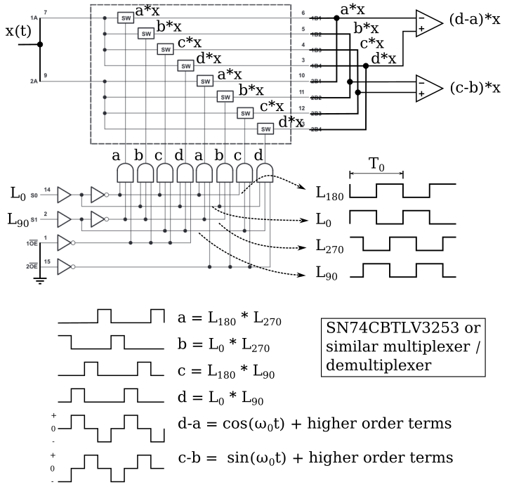
The LO outputs are fed into the select inputs S0 and S1 of the multiplexer chip, while the input signal \(x(t)\) is connected to both channel common points 1A and 2A. The switch control logic uses a combination of the LO signals and their inverses to route \(x(t)\) to two different I/O channels during each quarter of an LO clock cycle. Using the LO-derived digital signals to turn \(x(t)\) on or off has the effect of multiplying \(x(t)\) by the LO clock, which is the second thing we needed in the list that started this section.

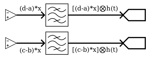
Op-amps connected to the I/O channels produce the difference in voltage between particular channels. These channels are selected to result in combinations that multiply \(x(t)\) with signals that look even more sinusoidal, \(d(t)-a(t) \approx \cos(\omega_0 t) + \text{higher order terms}\) and \(c(t)-b(t) \approx \sin(\omega_0 t) + \text{higher order terms}\). What are these higher order terms? While it is possible to use Fourier analysis to work out their precise amplitudes, all we need to know for our purposes is that they will be at every harmonic of \(\omega_0\), generally getting weaker at higher harmonics. Put mathematically:

\[d(t)-a(t) = a_0 \cos(\omega_0 t) + a_1 \cos(2\omega_0 t) + a_2 \cos(3\omega_0 t) + ...\]

We will need to use filtering to remove these higher-order terms. Let’s walk through the signals in the time and frequency domain to satisfy ourselves that it works.

First, take a look at the rest of the circuit. The outputs of the op-amps are filtered by fixed-frequency anti-aliasing filters and then digitized.

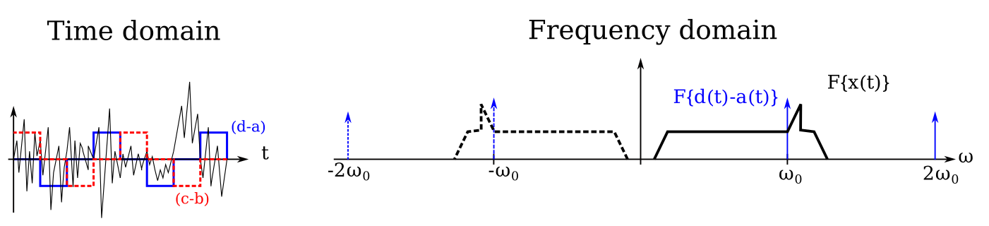
Now let’s look at the signals in the plot below. The signal \(x(t)\) is again shown as some arbitrary noisy wave containing a broad range of frequencies that span our actual band of interest, which is the little peak in the spectrum. I’ve included the first of undesirable higher order terms of the LO in the frequency domain plot. I’ve omitted \(F\{ c(t)-b(t) \}\) for simplicity in the drawing, but it’ll look like the example from the Quadrature Mixer section above.

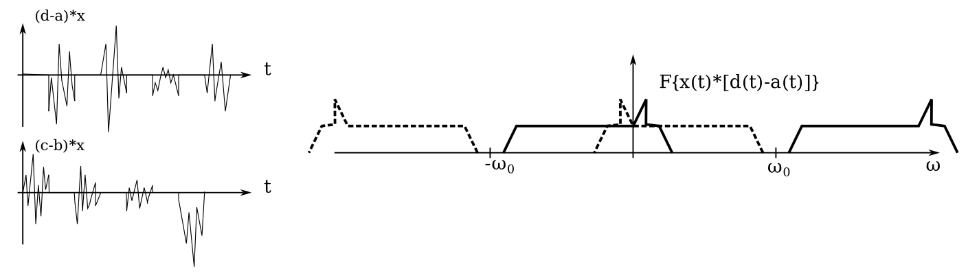
The output of the mixer looks like the plot below. The \(x(t)\) signal is present in one of the two mixer outputs at any given time, and is multiplied by -1 when \(d-a\) or \(c-b\) are negative. In the Fourier domain we see the effect of the undesired higher-order terms of the LO frequency: there are additional images of the positive and negative frequencies repeated outward (theoretically) infinitely along frequency axis.

Fortunately, the anti-aliasing filters remove these undesired higher-frequency signals. Shown in the plot below is the effect of filtering on the \((d-a)(t)x(t)\) signal. It neatly removes all the undesired signals leaving a clean signal ready for digitization at some sample rate \(\omega_s\). The \((c-b)(t)x(t)\) signal will look similar, except with a phase shift between the positive and negative frequency images as in the quadrature mixer discussion above.

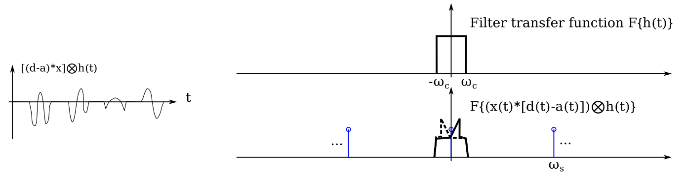
And that’s how a QSD works.

A real schematic

Here’s a real QSD schematic, derived from the excellent T41 software-defined transceiver. A pdf version can be downloaded here.

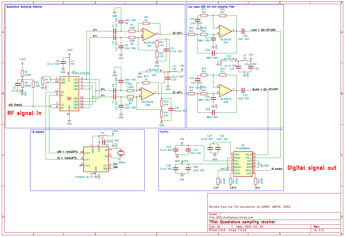
This implementation uses a cheap, high quality stereo audio digitizer PCM1808 to digitize the output. It reduces the signal bandwidth from the ~400 kHz produced by the anti-aliasing filters to 192 kHz. Remember that because we’re doing quadrature sampling we get a digital signal bandwidth that is twice the sample rate without violating the Nyquist limit. Think of it this way: in simple mixing you need to digitize one channel at twice the highest frequency, in quadrature sampling you digitize two channels at half the rate. Both methods produce the same amount of data to represent the same input signal bandwidth.