What is the T41?

The T41-EP Software Defined Transceiver (SDT), originally designed by Al Peter-AC8GY and Jack Purdum-W8TEE, is a 20W, HF, 7 band, CW/SSB Software Defined Transceiver (SDT) with a rich feature set. The T41-EP is a self-contain SDT that does not require an external PC, laptop, or tablet to use.

The T41-EP is a fully open-source radio. The repository for the transceiver software is hosted on GitHub. The hardware designs are hosted on Bill-K9HZ’s GitHub repository. The primary forum for discussions on the T41-EP radio is on Groups.io.

This post is a detailed write-up of the error model and calibration approach for the T41 V12 radio.

RF board design

A block diagram view of the T41’s V12 RF board is shown below. The receive chain is shown along the upper portion of the block diagram: the RF signal from the antenna enters through J2 and is amplified by U2 before being mixed by quadrature mixer U1 (see this post for an explanation of the mixer). After gain and filtering stages, the I and Q intermediate frequency (IF) channels leave the RF board through J1 to a PCM1808 ADC on the main board where they are digitized. The rest of the signal processing happens in the DSP chain.

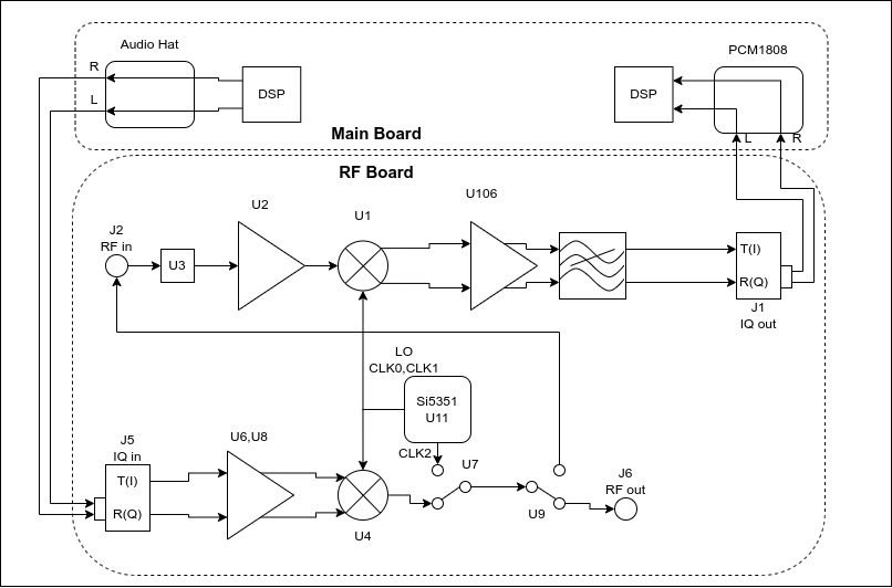
The transmit chain is shown along the bottom. The I/Q signals to be transmitted are generated by the Teensy audio hat and enter the RF board through J5. They are amplified and phased by U6 and U8, mixed by U4, and leave the RF board through J6.

A key feature of the T41 V12 RF board is that the transmit and receive chains share the same local oscillator: an Si5351 clock generator (U11) that produces quadrature outputs on CLK0 and CLK1.

The RF board has two more features that help us calibrate the board:

1. The signal produced by the transmit chain can be routed to the receive chain by controlling RF switch U9. This allows the T41 to examine its own transmit signal.
2. The third clock output of the Si5351, CLK2, can be routed into the transmit signal path using U7, and then into the receive path using U9. This allows us to use the Si5351 as an internal signal generator to measure the performance of the receive circuit.

Receive chain imperfections

Gain and phase differences between the I and Q signal paths in the T41 V12 receiver result in improper separation of the sidebands. To measure these differences we place the T41 RF board into the configuration shown below:

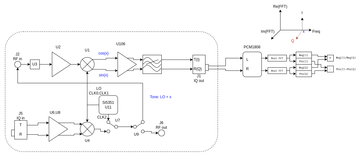
1. First, we set the CLK2 output of the Si5351 to be at some frequency \(x\) close to the LO frequency.
2. Route the CLK2 output into the receive chain using U7 and U9.
3. In the DSP chain, calculate FFTs of the L and R channels (I and Q respectively).
4. Find the CLK2 tone in the spectrum and measure its amplitude and phase in both the L and R (I and Q) channels.
5. Compute the ratio of the amplitude of the tone as seen in the L and R channels, and the phase difference between them.

If the receiver were perfect, we would expect the amplitude ratio to be 1, i.e., the CLK2 tone has been received with equal amplitude in the I and Q channels. We expect the phase difference to be \(\pm 90^\circ\), depending on whether the tone is in the lower sideband (\(-90^\circ\)) or upper sideband (\(+90^\circ\)).

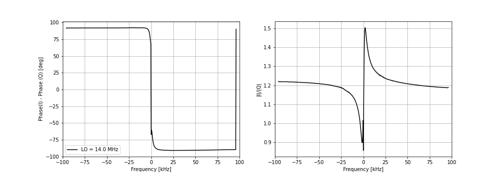
By sweeping \(x\) across the band and measuring the ratios and differences at each point in the sweep, we find the phase and amplitude balance between the I and Q channels to be something like this:

The T41 code contains a routine for performing this measurement called “IQ Balance” under the “Calibrate” menu.

Over most of the IF band, the phase balance is close to the ideal values. The amplitude balance is worse for the board under test: it deviates substantially from 1 over almost the entire IF band.

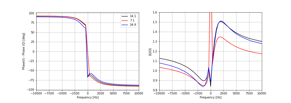
How does the IQ balance vary with LO frequency? It remains the same within a band, as shown by these measurements taken at three frequencies 14.0 MHz, 14.1 MHz, and 14.2 MHz in the 20m band.

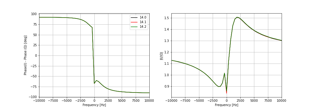
But it varies between bands, as shown by these measurements taken in the 20m (14.1 MHz), 40m (7.1 MHz), and 12m (24.9 MHz) bands:

Receive error model

We characterize the imperfections in the receive chain using two parameters, \(g(\omega_{IF})\) and \(\phi(\omega_{IF})\), that vary with the IF frequency \(\omega_{IF} = 2\pi(f_{\rm tone}-f_{\rm LO})\). \(f_{\rm tone}\) is the frequency generated by the CLK2 output of the Si5351 while \(f_{\rm LO}\) is the LO frequency generated by the CLK0 and CLK1 outputs.

The signals seen at frequency \(\omega_{IF}\) on the I and Q channels are given by:

\[I(\omega_{IF}) = g(\omega_{IF}) A_t \cos(\omega_{IF}t + \pi/2) + g(-\omega_{IF}) A_i \cos(-\omega_{IF}t - \pi/2)\] \[Q(\omega_{IF}) = A_t \cos\big(\omega_{IF}t + \phi(\omega_{IF})\big) + A_i \cos\big(-\omega_{IF}t + \phi(-\omega_{IF})\big)\]

In the case of an ideal receiver, \(g=1\) and \(\phi=0\), so our I and Q outputs are:

\[I(\omega_{IF}) = A_t \cos(\omega_{IF}t + \pi/2) + A_i \cos(-\omega_{IF}t - \pi/2)\] \[Q(\omega_{IF}) = A_t \cos(\omega_{IF}t ) + A_i \cos(-\omega_{IF}t)\]

Here \(A_i\) is the amplitude of the signal at the image frequency, while \(A_t\) is the amplitude of the signal at the tone frequency \(f_{\rm tone}\). In the DSP chain we make a complex number from the I and Q values that is then used through all the subsequent processing steps:

\[-I + jQ = 2 A_t \cos(\omega_{IF}t)\]

So we see that in a perfect receiver the signals from the image frequency \(-\omega_{IF}\) are perfectly canceled when we form the complex number \(-I + jQ\) and don’t appear in the output. This is perfect sideband separation.

To compensate for the errors in an imperfect receiver, we could multiply \(I(\omega_{IF})\) by \(1/g(\omega_{IF})\) to remove the gain imbalance, and apply a phase shift to \(Q(\omega_{IF})\) to remove the phase imbalance. How do we actually go about doing this?

Most correct calibration method

\(g\) and \(\phi\) vary with frequency, so the most correct way to apply the calibration is to do so in the frequency domain. In this method, we transform the time samples into the frequency domain and apply a different gain correction and phase rotation to every bin in the frequency domain, as shown by this code snippet:

import numpy as np
# L and R are numpy arrays of floats containing the time samples 
# from the left and right channels respectively. correctionG and
# correctionP are the pre-calculated gain correction and phase
# shift correction

# Transform L and R to the frequency domain
FL =  np.fft.fft(L)
FR =  np.fft.fft(R)
for k in range(len(FL)):
    # Apply the gain correction
    FL[k] = FL[k] / correctionG[k]
    # Apply the phase rotation
    a = np.real(FR[k])
    b = np.imag(FR[k])
    rr = np.cos(correctionP[k])
    ri = np.sin(correctionP[k])
    FR[k] = (a*rr - b*ri) + 1j*(b*rr + a*ri)
# Transform L and R back to the time domain
Lc = np.fft.ifft(FL)
Rc = np.fft.ifft(FR)
#  Lc and Rc are complex numbers, do some complex math. Numpy has a 
# complex data type that would make this simpler, but being explicit
# so it's easier to port this code to C.
a = np.real(Lc)
b = np.imag(Lc)
c = np.real(Rc)
e = np.imag(Rc)
IQc = -(a-e) + 1j*(b+c)

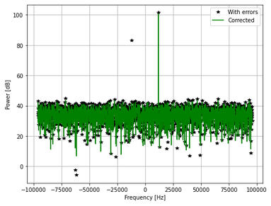
The efficacy of this technique when applied to simulated data is shown in the plot below. Without the calibration corrections, the tone at +10 kHz leaks into its image frequency frequency -10 kHz. If we apply the corrections, the sideband leakage is entirely eliminated.

However, this method is computationally expensive and memory intensive. We need to perform four additional FFTs on every block of data: two FFTs to transform to the frequency domain and two more to transform back to the time domain. We also need to store two 32-bit float values in memory for every frequency bin and allocate enough RAM for the outputs of the FFTs. In the T41 we typically act on blocks of 2048 samples, so the correction values need 16,384 bytes of RAM and the FFTs need 32,768 bytes (assuming we perform the FFTs in-place: 2 FFTs x 4 bytes x 2 numbers (real+complex) x 2048 samples).

Most efficient method

While the method above is the most correct and will perfectly calibration the data across the entire IF band, it is unnecessarily complicated. After all, we only demodulate a few kHz of bandwidth in the audio processing chain. This allows us to drastically simplify the calibration approach.

The T41 audio processing chain demodulates the portion of the electromagnetic spectrum that is about 48 kHz below the LO frequency (see FFTShift1 function in Freq_Shift.cpp).

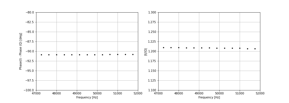
Let’s look at the gain and phase imbalances over a narrow bandwith 48 kHz above the IF frequency - this is the signal that we want to prevent from leaking into the demodulated audio in the signal processing chain. We see that the phase imbalances are almost constant over this band.

So, because we restrict our demodulation signal processing to a narrow part of the IF band, we only need to store a single gain correction and a single phase correction value for the whole band.

This simplification allows us to avoid the computational complexity too. We no longer need to perform the FFTs since we apply frequency-invariant amplitude and phase corrections. The T41 code applies an amplitude correction to the L buffer (the I channel):

arm_scale_f32 (float_buffer_L, -IQAmpCorrectionFactor[currentBand], float_buffer_L, BUFFER_SIZE * N_BLOCKS);

And applies something that approximates a phase correction:

void IQPhaseCorrection(float32_t *I_buffer, float32_t *Q_buffer, float32_t factor, uint32_t blocksize) {
  float32_t temp_buffer[blocksize];
  if (factor < 0.0) {  // mix a bit of I into Q
    arm_scale_f32(I_buffer, factor, temp_buffer, blocksize);
    arm_add_f32(Q_buffer, temp_buffer, Q_buffer, blocksize);
  } else {  // mix a bit of Q into I
    arm_scale_f32(Q_buffer, factor, temp_buffer, blocksize);
    arm_add_f32(I_buffer, temp_buffer, I_buffer, blocksize);
  }
}

Transmit calibration: If only it were that simple

A feature of the V12 hardware that makes it cheaper to build - its use of a single shared Si5351 between the transmit and receive channels - makes the transmit calibration procedure more complicated.

During the transmit calibration procedure we want to correct for I/Q imbalances at audio frequencies in the transmit chain. We do this by generating a 750 Hz audio tone. Take a look at what happens when we do this:

The 750 Hz transmit audio tone ends up around the 0 Hz IF frequency where the performance of the receiver is at its worst. A detailed measurement of the IQ balance looks like this:

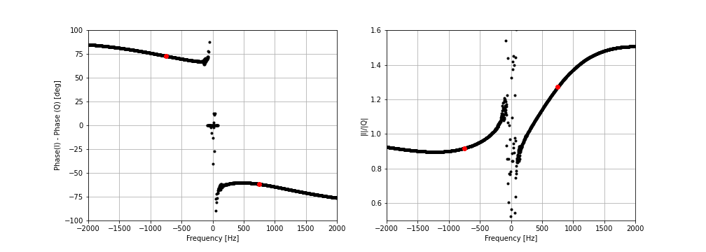
The phase and amplitude imbalances are changing rapidly with frequency. In principle, the same simplified method we use in the receive calibration above should work. In practice, we find that this method cannot sufficiently reduce the receive errors, likely because power from the LO leaks into the output and mixes with the tone in later parts of the signal chain to produce additional “false” power at the image frequency.

Receive Calibration Process

When in the receive calibration state, the front panel buttons are mapped as follows:

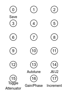
Receive calibration steps:

1. Enter receive calibration state by selecting Menu -> Calibrate -> Rec Cal.
2. Press Autotune button to find the best sideband separation.
3. Once autotune completes, press Save button to save values to EEPROM.

You can experiment with changes the values manually using the Filter encoder. Press the Gain/Phase button to switch between changing the amplitude correction and the phase correction and press the Increment button to change the increment value.

If the receive signal level is too high, you can adjust the attenuation levels of the transmit and receive attenuators. Rotating the Fine Tune encoder will change the attenuation level; press the Toggle Attenuator button (15) to select which attenuator is changed by the encoder.

You can examine the RF signal being produced by the Si5351 by pressing the J6/J2 button to toggle U9.

Transmit Calibration Process

The button mapping when in transmit calibration state is:

Currently, transmit calibration must be performed using an external spectrum analyzer.

1. Press the Xmit/Rec button to switch to Xmit calibrate.
2. Press the J6/J2 button to route the transmit signal to J6.
3. Place a spectrum analyzer on J6.
4. Manually tune the gain and phase to maximize sideband separation.